Hands-on Exercise 5E

Published

February 5, 2024

Modified

February 2, 2024

16 Treemap Visualisation

16.1 Overview and Learning Outcomes

This hands-on exercise is based on Chapter 16 of the R for Visual Analytics book.

The learning outcomes are:

Manipulate transaction data into a treemap stccuture using selected functions provided in the dplyr package.
Plot static treemaps using the treemap package.
Design interactive treemaps using the d3treeR package.

16.2 Getting Started

16.2.1 Installing and Loading Required Libraries

In this hands-on exercise, the following R packages are used:

tidyverse (i.e. readr, tidyr, dplyr) for performing data science tasks such as importing, tidying, and wrangling data;
treemap for plotting treemaps; and
d3treeR for plotting interactive treemaps.

The code chunk below uses the p_load() function in the pacman package to check if the packages are installed. If yes, they are then loaded into the R environment. If no, they are installed, then loaded into the R environment.

pacman::p_load(tidyverse, treemap,
               treemapify, d3treeR)

16.2.2 Importing Data

The dataset for this hands-on exercise is imported into the R environment using the read_csv() function in the readr package and stored as the R object, realis2018. The data contains information regarding private property transaction records in 2018 from the Urban Redevelopment Authority.

realis2018 = read_csv("data/realis2018.csv")

The tibble data frame, realis2018, has 20 columns and 23,205 rows.

16.2.3 Preparing Data

The data frame, realis2018, is in trasaction record form, which is highly disaggregated and not appropriate to be used to plot a treemap.

Hence, the raw data frame should be manipulated to prepre a suitable data frame by:

Grouping transaction records by “Project Name”, “Planning Region”, “Planning Area”, “Property Type”, and “Type of Sale”, and
Computing “Total Unit Sold”, “Total Area”, “Median Unit Price”, and “Median Transacted Price” by applying the appropriate summary statistics on “No. of Units”, “Area (sqm)”, “Unit Price ($ psm)”, and “Transacted Price ($)” respectively.

The following functions in the dplyr package would be used:

group_by() breaks down a data frame into specified groups of rows; and
summarise() computes the summary for each group.

Grouping affects the verbs as follows:

Grouped select() is the same as ungrouped select(), except that grouping variables are always retained.
Grouped arrange() is the same as ungrouped; unless “.by_group = TRUE” is set, in which case it orders first by the grouping variables.
mutate() and filter() are most useful in conjunction with window functions (like rank(), or min(x) == x). They are described in detail in vignette (“window-functions”).
sample_n() and sample_frac() sample the specified number/fraction of rows in each group.

realis2018_summarised = realis2018 %>% 
  group_by(`Project Name`,`Planning Region`, 
           `Planning Area`, `Property Type`, 
           `Type of Sale`) %>%
  summarise(`Total Unit Sold` = sum(`No. of Units`, na.rm = TRUE), 
            `Total Area` = sum(`Area (sqm)`, na.rm = TRUE),
            `Median Unit Price ($ psm)` = median(`Unit Price ($ psm)`, na.rm = TRUE),
            `Median Transacted Price` = median(`Transacted Price ($)`, na.rm = TRUE))

Note: Aggregation functions such as sum() and median() obey the usual rule of missing values: if there is any missing value in the input, the output will be a missing value. The “na.rm” argument set as “TRUE” removes the missing values prior to computation.

16.4 Designing Treemap: treemap Package

The treemap package is specially designed to offer great flexibility in drawing treemaps. The core function, treemap(), offers at least 43 arguments.

16.4.1 Designing Static Treemap

The treemap() function in the treemap package is used to plot a treemap to show the distribution of median unit prices and total unit sold of resale condominium by geographical hierarchy in 2017.

First, the records of resale condominium are selected using the filter() function in the dplyr package.

realis2018_selected = realis2018_summarised %>%
  filter(`Property Type` == "Condominium", `Type of Sale` == "Resale")

16.4.2 Using Basic Arguments

A basic treempa is plotted using the treemap() function, with the three core arguments of “index”, “vSize”, and “vColor”.

The “index” vector must consist of at least two column names or else no hierarchy treemap will be plotted. If multiple column names are provided, the first name is the highest aggregation level, the second name the second highest aggregation level, etc.
The “vSize” argument must be a column that does not contain negative values. This is because its values will be used to map the sizes of the rectangles of the treemaps.

treemap(realis2018_selected,
        index=c("Planning Region", "Planning Area", "Project Name"),
        vSize="Total Unit Sold",
        vColor="Median Unit Price ($ psm)",
        title="Resale Condominium by Planning Region and Area, 2017",
        title.legend = "Median Unit Price (S$ per sq. m)")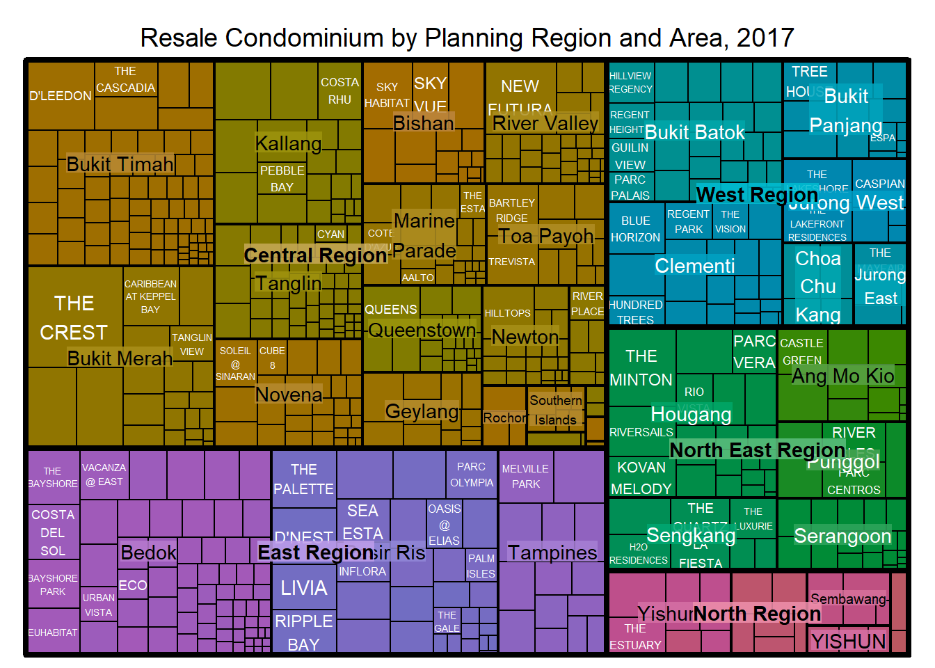

Note: The treemap above was wrongly coloured. For a correctly designed treemap, the colours of the rectangles should be in different intensity showing, in the case above, median unit prices. Hence, the “vColor” argument is used in combination with the “type” argument to determine the colours of the rectangles. Without defining the “type” argument, it is assumed that “type = index”, in the case above, the hierarchy of planning areas.

16.4.3 Working with vColor and type Arguments

Hence, the “type” argument set as “value” is added.

The rectangles are then coloured with different intensities of green, reflecting their respective median unit prices. The legend reveals that the values are binned into ten bins (i.e. 0-5000, 5000-10000, etc.) with an equal interval of 5000.

treemap(realis2018_selected,
        index=c("Planning Region", "Planning Area", "Project Name"),
        vSize="Total Unit Sold",
        vColor="Median Unit Price ($ psm)",
        type = "value",
        title="Resale Condominium by Planning Region and Area, 2017",
        title.legend = "Median Unit Price (S$ per sq. m)"        )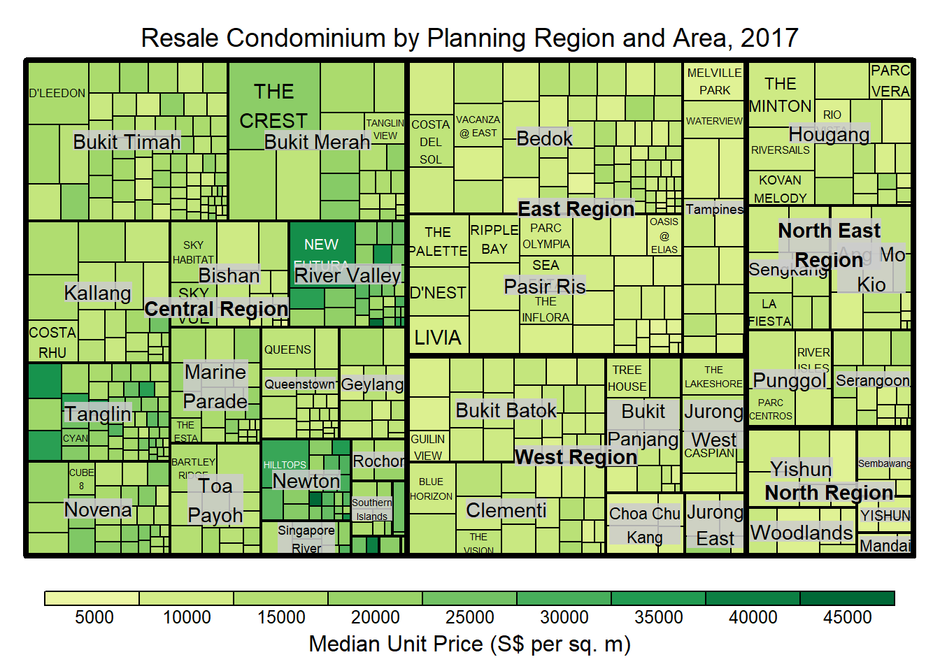

16.4.4 Colours in treemap Package

There are two arguments that determine the mapping to colour palettes: “mapping”, and “palette”. The only difference between “value” and “manual” is the default value for mapping.

The “value” treemap considers palette to be a diverging color palette (e.g., ColorBrewer’s “RdYlBu”), and maps it in such a way that 0 corresponds to the middle color (typically white or yellow), -max(abs(values)) to the left-end color, and max(abs(values)), to the right-end color.
The “manual” treemap simply maps min(values) to the left-end color, max(values) to the right-end color, and mean(range(values)) to the middle color.

16.4.5 “Value” Type treemap

A “value” type treemap is plotted below.

Although the colour palette used is RdYlBu but there are no red rectangles in the treemap because all the median unit prices are positive. The reason why we see only 5000 to 45000 in the legend is because the range argument is by default c(min(values, max(values)) with some pretty rounding.

treemap(realis2018_selected,
        index=c("Planning Region", "Planning Area", "Project Name"),
        vSize="Total Unit Sold",
        vColor="Median Unit Price ($ psm)",
        type="value",
        palette="RdYlBu", 
        title="Resale Condominium by Planning Region and Area, 2017",
        title.legend = "Median Unit Price (S$ per sq. m)"        )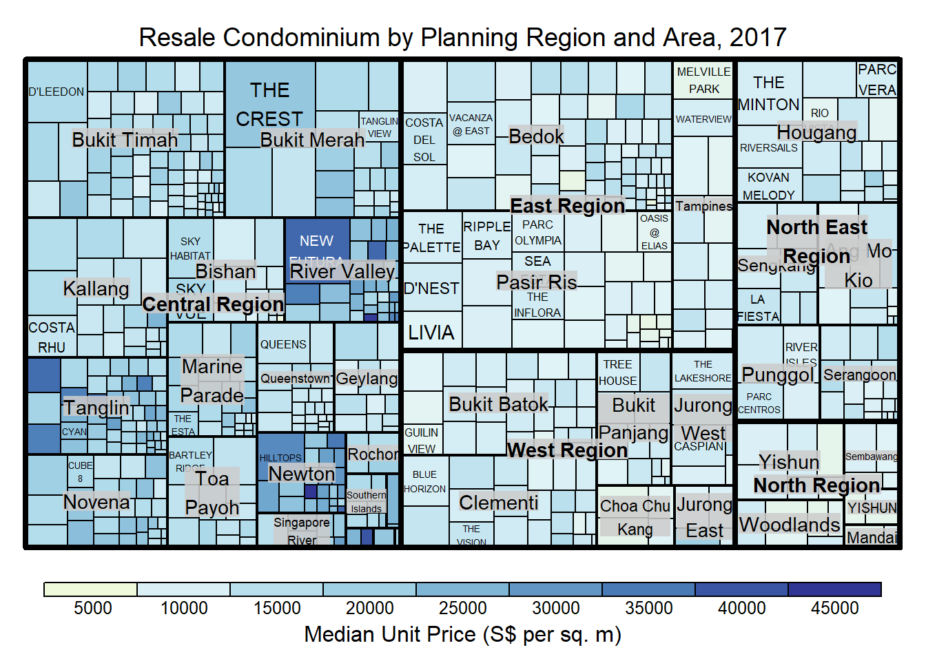

16.4.6 “Manual” Type treemap

The “manual” type does not interpret the values as the “value” type does. Instead, the value range is mapped linearly to the colour palette.

The colour scheme used is very confusing because mapping = (min(values), mean(range(values)), max(values)). It is not wise to use diverging colour palette such as RdYlBu if the values are all positive or negative.

treemap(realis2018_selected,
        index=c("Planning Region", "Planning Area", "Project Name"),
        vSize="Total Unit Sold",
        vColor="Median Unit Price ($ psm)",
        type="manual",
        palette="RdYlBu", 
        title="Resale Condominium by Planning Region and Area, 2017",
        title.legend = "Median Unit Price (S$ per sq. m)")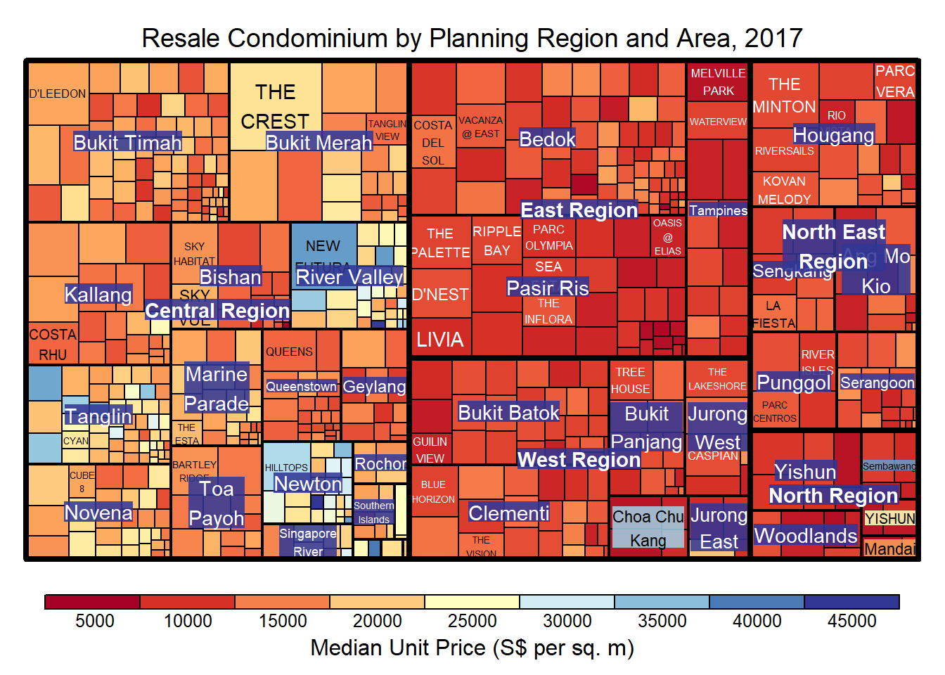

A single colour palette such as Blues is used instead.

treemap(realis2018_selected,
        index=c("Planning Region", "Planning Area", "Project Name"),
        vSize="Total Unit Sold",
        vColor="Median Unit Price ($ psm)",
        type="manual",
        palette="Blues", 
        title="Resale Condominium by Planning Region and Area, 2017",
        title.legend = "Median Unit Price (S$ per sq. m)")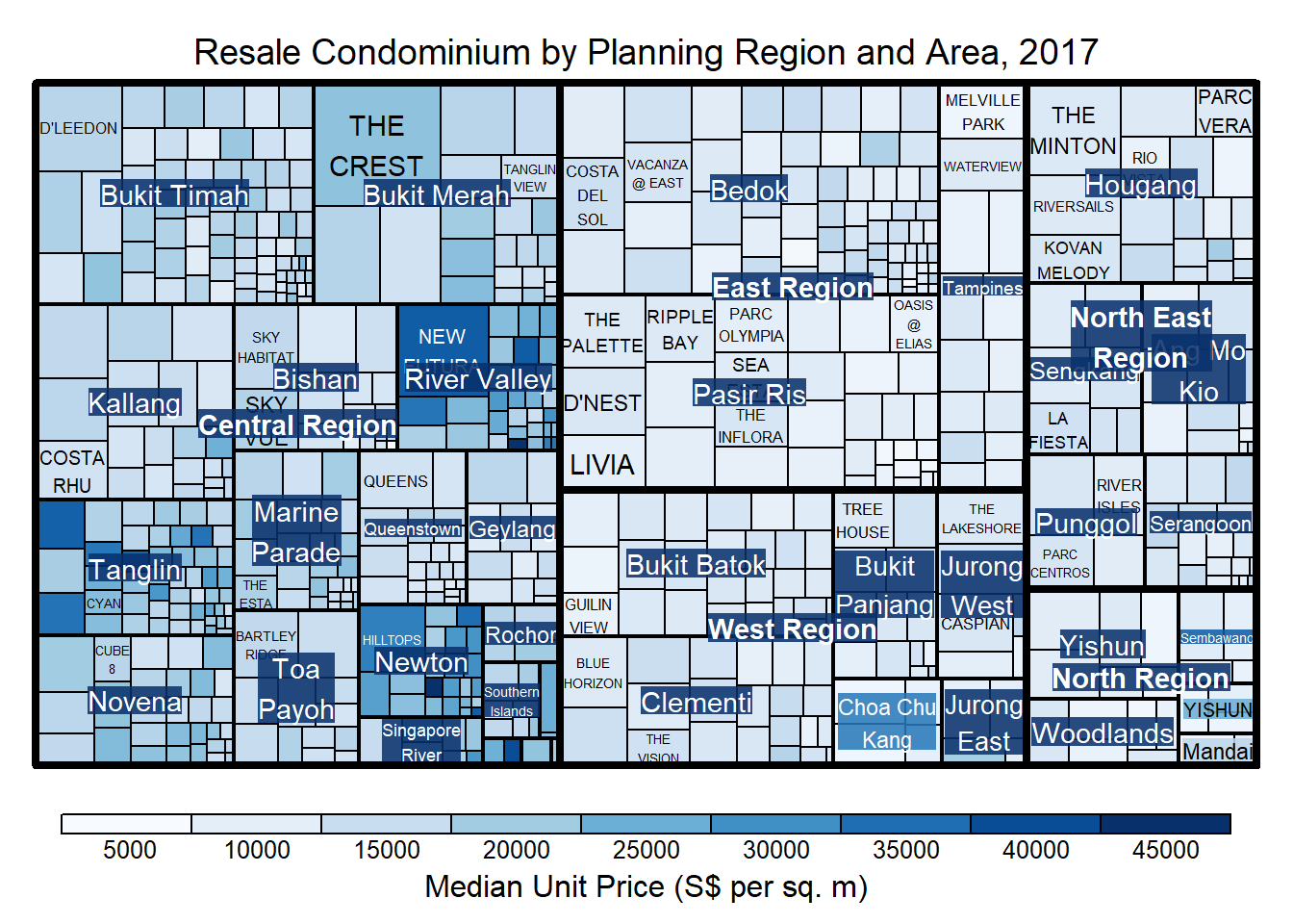

16.4.7 Treemap Layout

The treemap() function supports two popular treemap layouts: “squarified”, and “pivotSize”. The default is “pivotSize”.

The squarified treemap algorithm (Bruls et al., 2000) produces good aspect ratios, but ignores the sorting order of the rectangles (sortID).
The ordered treemap, pivot-by-size, algorithm (Bederson et al., 2002) takes the sorting order (sortID) into account while aspect ratios are still acceptable.

16.4.8 Working with algorithm Argument

A squarified treemap is plotted by changing the “algorithm” argument.

treemap(realis2018_selected,
        index=c("Planning Region", "Planning Area", "Project Name"),
        vSize="Total Unit Sold",
        vColor="Median Unit Price ($ psm)",
        type="manual",
        palette="Blues", 
        algorithm = "squarified",
        title="Resale Condominium by Planning Region and Area, 2017",
        title.legend = "Median Unit Price (S$ per sq. m)")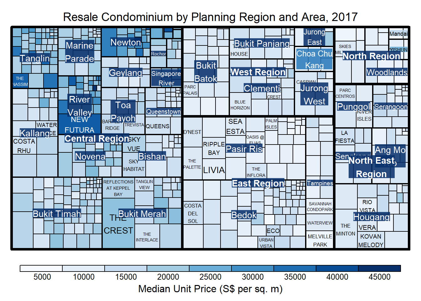

16.4.9 Using sortID Argument

When the “pivotSize” algorithm is used, the “sortID” argument can be used to dertemine the order in which the rectangles are placed from top left to bottom right.

treemap(realis2018_selected,
        index=c("Planning Region", "Planning Area", "Project Name"),
        vSize="Total Unit Sold",
        vColor="Median Unit Price ($ psm)",
        type="manual",
        palette="Blues", 
        algorithm = "pivotSize",
        sortID = "Median Transacted Price",
        title="Resale Condominium by Planning Region and Area, 2017",
        title.legend = "Median Unit Price (S$ per sq. m)")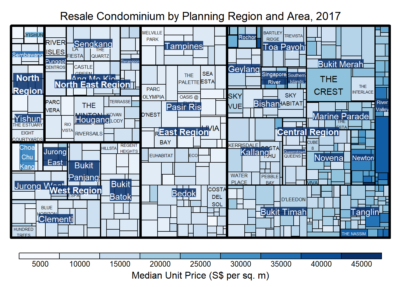

16.5 Designing Treemap: treemapify Package

The treemapify package is specially developed to draw treemaps in ggplot2.

16.5.1 Designing Basic Treemap

ggplot(data=realis2018_selected, 
       aes(area = `Total Unit Sold`,
           fill = `Median Unit Price ($ psm)`),
       layout = "scol",
       start = "bottomleft") + 
  geom_treemap() +
  scale_fill_gradient(low = "light blue", high = "blue")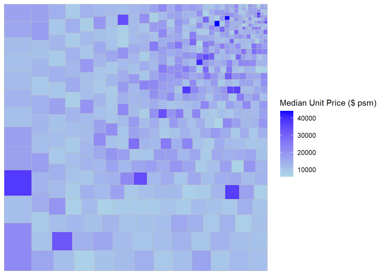

16.5.2 Defining Hierarchy

The treemap is plotted by grouping by “Planning Region”.

ggplot(data=realis2018_selected, 
       aes(area = `Total Unit Sold`,
           fill = `Median Unit Price ($ psm)`,
           subgroup = `Planning Region`),
       start = "topleft") + 
  geom_treemap()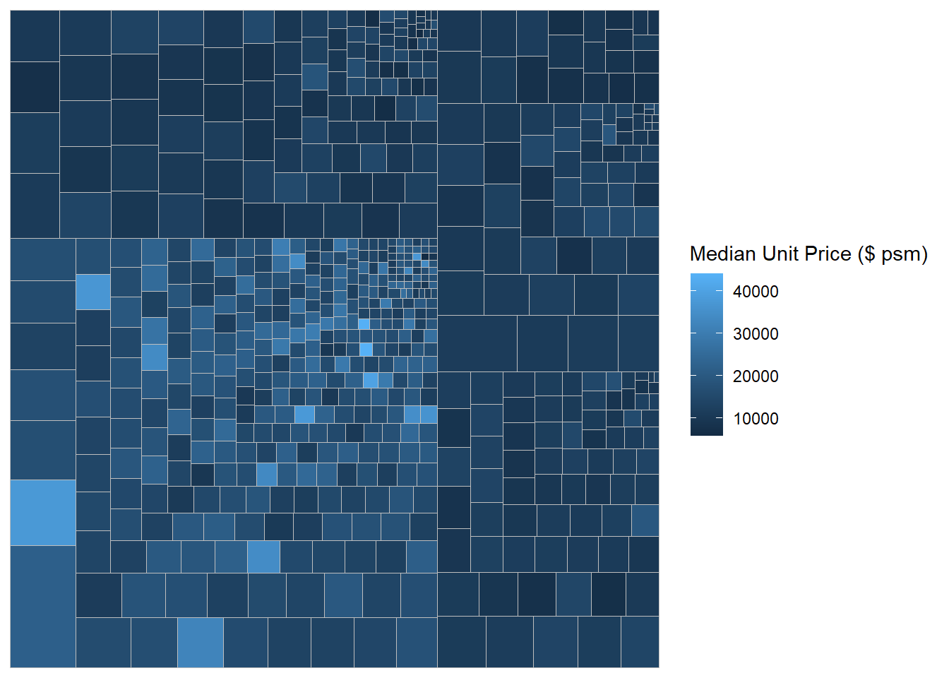

The treemap is plotted by further grouping by “Planning Area”.

ggplot(data=realis2018_selected, 
       aes(area = `Total Unit Sold`,
           fill = `Median Unit Price ($ psm)`,
           subgroup = `Planning Region`,
           subgroup2 = `Planning Area`)) + 
  geom_treemap()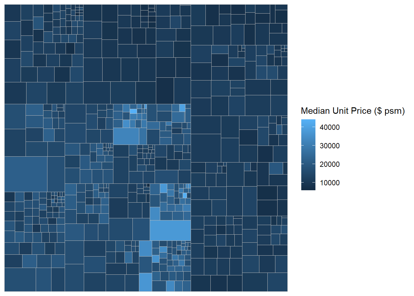

Boundary lines are then added.

ggplot(data=realis2018_selected, 
       aes(area = `Total Unit Sold`,
           fill = `Median Unit Price ($ psm)`,
           subgroup = `Planning Region`,
           subgroup2 = `Planning Area`)) + 
  geom_treemap() +
  geom_treemap_subgroup2_border(colour = "gray40",
                                size = 2) +
  geom_treemap_subgroup_border(colour = "gray20")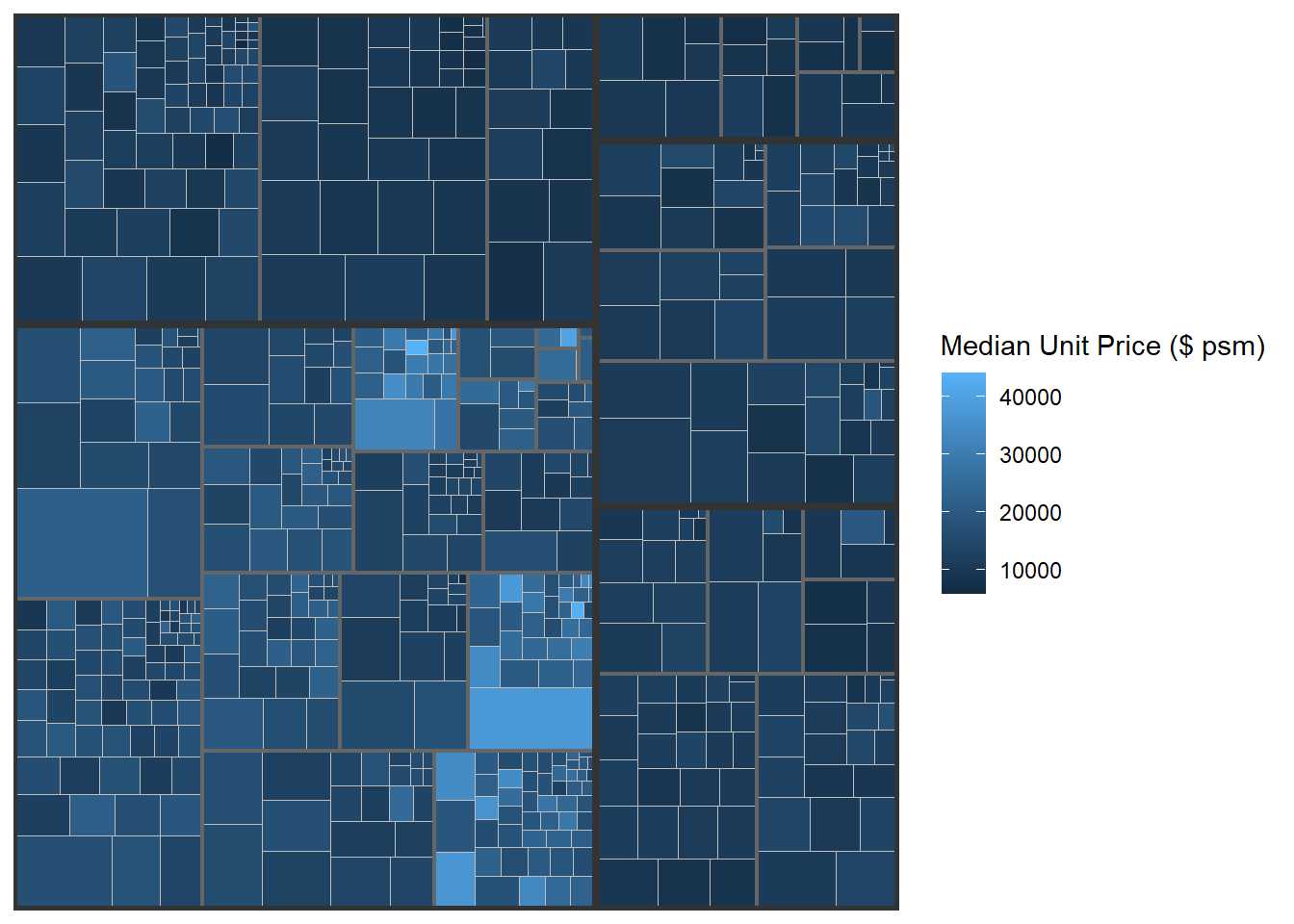

16.6 Designing Interactive Treemap: d3treeR Package

An interactive treemap is created using two steps:

First, the treemap() function is used to build a treemap, tm, using the selected variables.

tm = treemap(realis2018_summarised,
        index=c("Planning Region", "Planning Area"),
        vSize="Total Unit Sold",
        vColor="Median Unit Price ($ psm)",
        type="value",
        title="Private Residential Property Sold, 2017",
        title.legend = "Median Unit Price (S$ per sq. m)")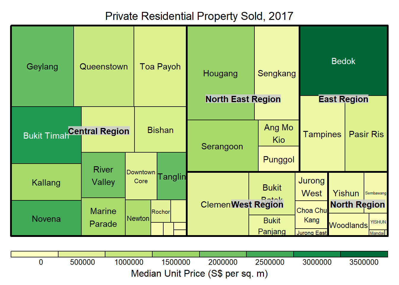

Then, the d3tree() function is used to build an interactive treemap.

d3tree(tm,rootname = "Singapore" )

~~~ End of Hands-on Exercise 5E ~~~